Note: knowing intermediate probability and calculus is necessary to understand this post.
Last week, I completed a summer course at Stanford: CS109, Probability for Computer Scientists. This 8-week long class was intense and challenging but one of the most rewarding classes I’ve taken at Stanford so far. A few weeks ago, I had an idea for a homework problem but I couldn’t quite figure out how to implement the idea. The problem is as follows:
Below are two sequences of 300 “coin flips” (H for heads, T for tails). One of these is a true sequence of 300 independent flips of a fair coin. The other was generated by a person typing out H’s and T’s and trying to seem random. Which sequence is the true sequence of coin flips? Make an argument that is justified with probabilities calculated on the sequences. Both sequences have 148 heads, two less than the expected number for a 0.5 probability of heads.
Sequence 1:
TTHHTHTTHTTTHTTTHTTTHTTHTHHTHHTHTHHTTTHHTHTHTTHTHH
TTHTHHTHTTTHHTTHHTTHHHTHHTHTTHTHTTHHTHHHTTHTHTTTHH
TTHTHTHTHTHTTHTHTHHHTTHTHTHHTHHHTHTHTTHTTHHTHTHTHT
THHTTHTHTTHHHTHTHTHTTHTTHHTTHTHHTHHHTTHHTHTTHTHTHT
HTHTHTHHHTHTHTHTHHTHHTHTHTTHTTTHHTHTTTHTHHTHHHHTTT
HHTHTHTHTHHHTTHHTHTTTHTHHTHTHTHHTHTTHTTHTHHTHTHTTT
Sequence 2:
HTHHHTHTTHHTTTTTTTTHHHTTTHHTTTTHHTTHHHTTHTHTTTTTTH
THTTTTHHHHTHTHTTHTTTHTTHTTTTHTHHTHHHHTTTTTHHHHTHHH
TTTTHTHTTHHHHTHHHHHHHHTTHHTHHTHHHHHHHTTHTHTTTHHTTT
THTHHTTHTTHTHTHTTHHHHHTTHTTTHTHTHHTTTTHTTTTTHHTHTH
HHHTTTTHTHHHTHHTHTHTHTHHHTHTTHHHTHHHHHHTHHHTHTTTHH
HTTTHHTHTTHHTHHHTHTTHTTHTTTHHTHTHTTTTHTHTHTTHTHTHTThere’s actually a straightforward approach to solving this problem that involves the geometric distribution, but after researching ways to approach this problem, I stumbled across something known as the Wald–Wolfowitz runs test (or simply runs test). According to Wikipedia, this is a “statistical test that checks a randomness hypothesis for a two-valued data sequence. More precisely, it can be used to test the hypothesis that the elements of the sequence are mutually independent.” In layman’s terms, it can be used to test the randomness of a distribution comprised of only two possible outcomes (heads and tails for example).
Intuitively, if someone flips a coin 10 times and gets 5 heads and 5 tails, it is more plausible that the order of outcomes H, T, T, H, T, H, H, H, T, T is more likely to be random than something like H, H, H, H, H, T, T, T, T, T. The runs test can analyze both experiments to see which one is more likely to be a truly random outcome of flips. By calculating the expectation (mean) and variance of the number of runs in this type of experiment, we can use the normal distribution to approximate the probability that we get a certain number of runs. We use the word “runs” to denote consecutive outcomes of the same result.
I was on a mission to find the expectation and variance for this problem. The expectation formula was simple to solve in a matter of minutes, but for some reason, I couldn’t find a proof of the variance anywhere on the internet (after an hour of searching). Every source I found cited textbooks that I do not have easy access to (this should be remedied once I’m an official Masters student this fall). I did, however, find a PDF of a book written in 1940 by the very people that the runs test is named after: “On a test whether two samples are from the same population”, by Wald and Wolfowitz. Excited to finally have the source of this test right at my fingertips, I began skimming the pages. To my disappointment, the authors decided to not reveal the “tedious calculations”:
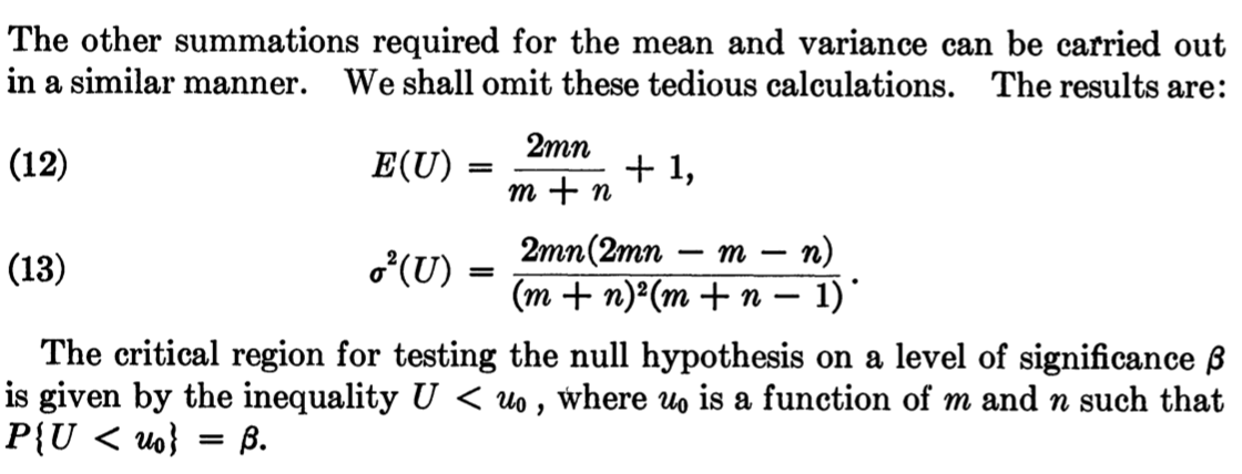
Wald, A.; Wolfowitz, J. On a Test Whether Two Samples are from the Same Population. Ann. Math. Statist. 11 (1940), no. 2, 147–162. doi:10.1214/aoms/1177731909. https://projecteuclid.org/euclid.aoms/1177731909.
*Blank stare*. I’m really curious to find out where exactly they proved these equations. Sigh. Thus I was left on my own to figure it out. I tried over several days to wrap my head around this problem, and it wasn’t until after finishing the class that I finally was able to approach the problem with a clear head. Here is my approach.
Let  be the number of runs (consecutive outcomes of the same result) in a series of coin tosses that result in
  heads and
  tails. We will find the equations for the expectation and variance of .
First, we will find the expected number of runs. Define  to be an indicator variable that represents whether the
  coin flip result does not equal the
  coin flip result. For any positive number of coin tosses, we can count the number of times the outcome switches to a different result. Since the second run counts as the first switch, we add 1 to the equation below to account for the first run, which defines the way the runs can alternate between heads and tails. For example,
  has 4 runs: 1 run of two heads followed by 3 switches (heads to tails, tails to heads, and heads to tails). We can now express R as 1 plus the sum of the indicator variables:

The summation starts from the first flip and goes to the second to last flip since we want to compare every flip to the flip that comes after it. Thus we compare the flips in every such pair. We can now express the expected number of runs when there are heads and tails as follows:
![\begin{align*} E[R] &= E \left[ 1 + \sum_{j=1}^{H+T-1}{I_j} \right] \end{align*}](https://www.rozmichelle.com/wp-content/ql-cache/quicklatex.com-766350fcd68fb38888839df304c2ab69_l3.png "Rendered by QuickLaTeX.com")
(Via linearity of expectation) ![\begin{align*} {\color{white}{E[R]}} &= E[1] + E \left[ \sum_{j=1}^{H+T-1}{I_j} \right] \end{align*}](https://www.rozmichelle.com/wp-content/ql-cache/quicklatex.com-04a74d12ad5137b6cb194f18c8d471bf_l3.png "Rendered by QuickLaTeX.com")
(Via linearity of expectation) ![\begin{align*} {\color{white}{E[R]}} = 1 + \sum_{j=1}^{H+T-1}{E \left[ I_j \right]} \end{align*}](https://www.rozmichelle.com/wp-content/ql-cache/quicklatex.com-a4823851202caaa32292fa5fe0ed2d27_l3.png "Rendered by QuickLaTeX.com")
Since the expected value of an indicator variable is simply the probability of the variable’s success, we have:
![\begin{align*} E[R] &= 1 + \sum_{j=1}^{H+T-1}{P \left( I_j = 1 \right)} \\ &= 1 + \sum_{j=1}^{H+T-1}{P \left( j^{th} flip \neq (j+1)^{th} flip \right)} \\ &= 1 + \sum_{j=1}^{H+T-1}{2 \left( \frac{H}{H+T} \frac{T}{H+T-1} \right)} \\ \end{align*}](https://www.rozmichelle.com/wp-content/ql-cache/quicklatex.com-19e4e5aedbed1104381c670c5b3cf7a2_l3.png "Rendered by QuickLaTeX.com")
We need the flip to be a different outcome than the flip that comes after it. If the flip is heads, there are ways to pick heads out of  outcomes, giving a probability
  that the flip is heads. After choosing one heads, there are
  remaining flips and T ways to choose tails out of those remaining flips. We lastly double this result since we have the same probability of having tails on the flip followed by heads. Simplifying gives:
![\begin{align*} E[R] &= 1 + \sum_{j=1}^{H+T-1}{ \frac{2HT}{(H+T)(H+T-1)} } \end{align*}](https://www.rozmichelle.com/wp-content/ql-cache/quicklatex.com-139d83d35de6fae1789bd031edcc0da8_l3.png "Rendered by QuickLaTeX.com")
(Since the body of the summation didn’t depend on j) ![\begin{align*} {\color{white}{E[R]}} &= 1 + (H+T-1) \frac{2HT}{(H+T)(H+T-1)} \end{align*}](https://www.rozmichelle.com/wp-content/ql-cache/quicklatex.com-3299100054ceda3b864c94980de62dbe_l3.png "Rendered by QuickLaTeX.com")
![\begin{align*} {\color{white}{E[R]}} &= {\color{MidnightBlue}{1 + \frac{2HT}{H+T} }} \end{align*}](https://www.rozmichelle.com/wp-content/ql-cache/quicklatex.com-f6857aa24b4154f56821c0ed59f14486_l3.png "Rendered by QuickLaTeX.com")
Thus we have the expected number of runs when we have heads and tails.
To find the variance, we must compute ![Var(R)=E[R^2]-{(E[R])}^2](https://www.rozmichelle.com/wp-content/ql-cache/quicklatex.com-db38a3b0a82228d3dba2622120c24f0e_l3.png "Rendered by QuickLaTeX.com") . First, compute
. First, compute ![{(E[R])}^2](https://www.rozmichelle.com/wp-content/ql-cache/quicklatex.com-65c738a9537ba745c18fac7c7e5f1b05_l3.png "Rendered by QuickLaTeX.com") :
:
![\begin{align*} {(E[R])}^2 &= {\left( 1 + \frac{2HT}{H+T} \right)}^2 \\ &= 1 + \frac{4HT}{H+T} + {\left( \frac{2HT}{H+T} \right)}^2 \\ \end{align*}](https://www.rozmichelle.com/wp-content/ql-cache/quicklatex.com-4866677760dbe1c9d9e39437466edadd_l3.png "Rendered by QuickLaTeX.com")
To compute ![E[R^2]](https://www.rozmichelle.com/wp-content/ql-cache/quicklatex.com-85dd4b93901186ee4942db018a0e1367_l3.png "Rendered by QuickLaTeX.com") , we’ll first find
, we’ll first find  . Recall that
  . Thus:

(Substitution using equation for R) 
(Equation 1: Expansion of square of summation) 
We can split the square of the summation this way because the square of a summation represents all  pairs in the range 1 to , inclusive, where there are two cases we can consider: the case where
  (represented by the first summation) and the case where
  (represented by the second summation). To show why this works, consider a simple example:

Note that we can actually compute the square using the FOIL method as follows:

We can rearrange the terms to get the following:
(Equation 2) 
Notice that we can express these terms as the sum of two summations: a summation of squares and a summation of products of different-valued integer pairs:

This is like the trick we used earlier. At this point, we can also use another summation property to expand the latter summation:

(Equation 3) 
Notice that the last three terms shown at the end of Equation 2 each have a product of an integer and a larger integer. Thus we can represent these products as the summation shown in Equation 3, where we double the summation to account for symmetry (e.g.  ). We could’ve also reversed the inequality sign to achieve the same result. I arbitrarily chose
  .
.
We can now use this approach in our equation for (Equation 1):


(because I is an indicator variable) 
(Substitution using equation for R) 

Now we can compute :
![\begin{align*} \ E[R^2] &= E \left[ 3R - 2 + 2\sum_{j<k}^{H+T-1}I_j I_k \right] \end{align*}](https://www.rozmichelle.com/wp-content/ql-cache/quicklatex.com-c0fc102b8ff9f64334cbc46e67a19a8b_l3.png "Rendered by QuickLaTeX.com")
(Via linearity of expectation) ![\begin{align*} \ {\color{white}{E[R^2]}} &= 3E[R] - E[2] + 2E \left[ \sum_{j<k}^{H+T-1}I_j I_k \right] \end{align*}](https://www.rozmichelle.com/wp-content/ql-cache/quicklatex.com-109192e41afba984d1a98f199a055540_l3.png "Rendered by QuickLaTeX.com")
(Via linearity of expectation & substitution using equation for R) ![\begin{align*} \ {\color{white}{E[R^2]}} &= 3 \left( 1 + \frac{2HT}{H+T} \right) - 2 + 2\sum_{j<k}^{H+T-1}E \left[ I_j I_k \right] \end{align*}](https://www.rozmichelle.com/wp-content/ql-cache/quicklatex.com-a25fc0909258abdc7ad55fcad801c84e_l3.png "Rendered by QuickLaTeX.com")
![\begin{align*} \ {\color{white}{E[R^2]}} &= 1 + \frac{6HT}{H+T} + 2\sum_{j<k}^{H+T-1} P \left( I_j I_k = 1 \right) \end{align*}](https://www.rozmichelle.com/wp-content/ql-cache/quicklatex.com-624fe03a4040c96d6cab7e060c7018d0_l3.png "Rendered by QuickLaTeX.com")
(Both variables must = 1 in order for their product to = 1) ![\begin{align*} \ {\color{white}{E[R^2]}} &= 1 + \frac{6HT}{H+T} + 2\sum_{j<k}^{H+T-1} P \left( I_j = 1, I_k = 1 \right) \end{align*}](https://www.rozmichelle.com/wp-content/ql-cache/quicklatex.com-cf89cc8aeae169af7363b7d6e8385a8f_l3.png "Rendered by QuickLaTeX.com")
In order to find the probability that both indicator variables equal 1, let’s further split the summation into two cases. Either the indicator variables and  each refer to pairs of flips that overlap (meaning the second flip of (the
  flip) equals the first flip of
  ), or the two indicator variables represent pairs of flips that have no flips in common. Since these two outcomes have different probabilities, we split them into summations that cover each case separately. Let’s explore these cases in more depth.
Case 1: We consider all indicator variables that share a flip, starting with indicator variables that compare the first three flips and incrementing by one until we end the summation with indicator variables that compare the last three flips. For example, say we have the following outcomes of 6 coin flips:  . The following highlighted outcomes represent indicator variables that share an outcome, where the first two purple-colored outcomes are the outcomes compared in the first indicator variable and the last two purple-colored outcomes are the ones compared in the second indicator variable:
![\[{{\color{DarkOrchid} T}, {{\color{DarkOrchid} H}, {{\color{DarkOrchid} T}, H, H, T\]](https://www.rozmichelle.com/wp-content/ql-cache/quicklatex.com-e5e45fc958cf4ff001b53740e07a2723_l3.png "Rendered by QuickLaTeX.com")
![\[T, {{\color{DarkOrchid} H}, {{\color{DarkOrchid} T}, {{\color{DarkOrchid} H}, H, T\]](https://www.rozmichelle.com/wp-content/ql-cache/quicklatex.com-42d642f7128a1254312e5cbd282c6b82_l3.png "Rendered by QuickLaTeX.com")
![\[T, H, {{\color{DarkOrchid} T}, {{\color{DarkOrchid} H}, {{\color{DarkOrchid} H}, T\]](https://www.rozmichelle.com/wp-content/ql-cache/quicklatex.com-f88550fc518fca2394b086c9654437b9_l3.png "Rendered by QuickLaTeX.com")
![\[T, H, T, {{\color{DarkOrchid} H}, {{\color{DarkOrchid} H}, {{\color{DarkOrchid} T}\]](https://www.rozmichelle.com/wp-content/ql-cache/quicklatex.com-c263f5c86e4148ce1d91098fd53bef4a_l3.png "Rendered by QuickLaTeX.com")
This example makes it easier to see that the summation bounds go from  to
to  so we always have three outcomes to consider.
Case 2: We consider all indicator variables that do not share a flip, thus four flips are considered at a time. Let’s visualize this with our 6 coin flips example:
![\[{{{\color{DarkOrchid} T}, {{\color{DarkOrchid} H}, {{\color{RoyalBlue} T}, {{\color{RoyalBlue} H}, H, T\]](https://www.rozmichelle.com/wp-content/ql-cache/quicklatex.com-c772516e824dd6da7135b4bc23844da9_l3.png "Rendered by QuickLaTeX.com")
![\[{{{\color{DarkOrchid} T}, {{\color{DarkOrchid} H}, T, {{\color{RoyalBlue} H}, {{\color{RoyalBlue} H}, T\]](https://www.rozmichelle.com/wp-content/ql-cache/quicklatex.com-515b4b44bbdbb3bb1a586a6e67de310c_l3.png "Rendered by QuickLaTeX.com")
![\[{{{\color{DarkOrchid} T}, {{\color{DarkOrchid} H}, T, H, {{\color{RoyalBlue} H}, {{\color{RoyalBlue} T}\]](https://www.rozmichelle.com/wp-content/ql-cache/quicklatex.com-51c390b052500e4841c3069a2f73ef37_l3.png "Rendered by QuickLaTeX.com")
![\[{T, {{\color{DarkOrchid} H}, {{\color{DarkOrchid} T}, {{\color{RoyalBlue} H}, {{\color{RoyalBlue} H}, T\]](https://www.rozmichelle.com/wp-content/ql-cache/quicklatex.com-a010b1ea6e7f4f33ec0f8835452e3eba_l3.png "Rendered by QuickLaTeX.com")
![\[{T, {{\color{DarkOrchid} H}, {{\color{DarkOrchid} T}, H, {{\color{RoyalBlue} H}, {{\color{RoyalBlue} T}\]](https://www.rozmichelle.com/wp-content/ql-cache/quicklatex.com-aae9e65bce4c67b14afb7e9d344b2739_l3.png "Rendered by QuickLaTeX.com")
![\[{T, H, {{\color{DarkOrchid} T}, {{\color{DarkOrchid} H}, {{\color{RoyalBlue} H}, {{\color{RoyalBlue} T}\]](https://www.rozmichelle.com/wp-content/ql-cache/quicklatex.com-8bf63350b9508cf8fe071f32fd48db05_l3.png "Rendered by QuickLaTeX.com")
In this case, we can use a nested summation to ensure that and never refer to the same flip. The outer summation starts from . It ends at  to ensure there are always four outcomes to consider (two for each indicator variable). The inner summation starts at
  (to ensure that it doesn’t consider one of the two flips that considers), and it ends at
  (to allow to consider the last two flips).
Notice that these two cases along with the case we saw earlier (where an indicator variable is squared) are mutually exclusive and exhaustive: we’ve accounted for all possible pairs of flips that the two indicator variables can compare. Now that we understand the cases, let’s update our equation:
![\begin{align*} \ E[R^2] &= 1 + \frac{6HT}{H+T} + 2\sum_{j<k}^{H+T-1} P \left( I_j = 1, I_k = 1 \right) \end{align*}](https://www.rozmichelle.com/wp-content/ql-cache/quicklatex.com-5314e9a22cf887458d9f5a5121305042_l3.png "Rendered by QuickLaTeX.com")
![\begin{align*} {\color{white}{E[R^2]}} &= 1 + \frac{6HT}{H+T} + 2\left( \sum_{j = 1}^{H+T-2} P \left( I_j = 1, I_{j+1} = 1 \right) + \sum_{j = 1}^{H+T-3} { \sum_{k = j+2}^{H+T-1} P \left( I_j = 1, I_k = 1 \right) } \right) \\ \end{align*}](https://www.rozmichelle.com/wp-content/ql-cache/quicklatex.com-cfe63b467cd44116b81aeded3b72815e_l3.png "Rendered by QuickLaTeX.com")
(Equation 4) ![\begin{align*} {\color{white}{E[R^2]}} &= 1 + \frac{6HT}{H+T} + 2 \sum_{j = 1}^{H+T-2} P \left( I_j = 1, I_{j+1} = 1 \right) + 2 \sum_{j = 1}^{H+T-3} { \sum_{k = j+2}^{H+T-1} P \left( I_j = 1, I_k = 1 \right) } \end{align*}](https://www.rozmichelle.com/wp-content/ql-cache/quicklatex.com-b000a1f0beeae30578731c2e50be1dd6_l3.png "Rendered by QuickLaTeX.com")
Let’s first expand the probability for the first case, recalling that and share a flip. For both  and
and  to be true at the same time, flip
  must be different from flip
  , and flip must be different from flip
  (thus flip and must have the same outcome). This means that these three sequential flips are either
  or
or  , as expressed below:

![\begin{align*} {\color{white}{2 \sum_{j = 1}^{H+T-2} P \left( I_j = 1, I_{j+1} = 1 \right)}} &= 2 \sum_{j = 1}^{H+T-2} \textstyle{ \left[ \left( \frac{H}{H+T} \cdot \frac{T}{H+T-1} \cdot \frac{H-1}{H+T-2} \right) + \left( \frac{T}{H+T} \cdot \frac{H}{H+T-1} \cdot \frac{T-1}{H+T-2} \right) \right]} \end{align*}](https://www.rozmichelle.com/wp-content/ql-cache/quicklatex.com-e0678e087d9c8b9c69ed373299d2c182_l3.png "Rendered by QuickLaTeX.com")


(Since summation body didn’t depend on j) 
Plugging this back into Equation 4 gives us:
(Equation 5) ![\begin{align*} E[R^2] &= 1 + \frac{6HT}{H+T} + \frac{2HT(H+T-2)}{(H+T)(H+T-1)} + 2 \sum_{j = 1}^{H+T-3} { \sum_{k = j+2}^{H+T-1} P \left( I_j = 1, I_k = 1 \right) } \end{align*}](https://www.rozmichelle.com/wp-content/ql-cache/quicklatex.com-02c86b28fcbad2bda9b3d50b1b292fc8_l3.png "Rendered by QuickLaTeX.com")
Now let’s consider the case where the two indicator variables do not overlap. We compute the probability that the two flips represented by each indicator variable have one and one :

We multiply the probability of each pair of flips having different outcomes by 2 to account for either HT or TH being the outcome. Let’s simplify, first by pulling out the constants that don’t depend on or  :
:


At this point, we can split the summation:

Now let’s simplify by using the arithmetic series formula:


Let’s plug this back into equation 5:
![\begin{align*} E[R^2] &= \textstyle{ 1 + \frac{6HT}{H+T} + \frac{2HT(H+T-2)}{(H+T)(H+T-1)} + \frac{4HT(H-1)(T-1)}{(H+T)(H+T-1)} } \end{align*}](https://www.rozmichelle.com/wp-content/ql-cache/quicklatex.com-9c24fbb3f9682613820a77e7bd59c0f0_l3.png "Rendered by QuickLaTeX.com")
![\begin{align*} {\color{white}{E[R^2]}} &= 1 + \textstyle{ \frac{6HT(H+T-1) + 2HT(H+T-2) + 4HT(H-1)(T-1)}{(H+T)(H+T-1)} } \end{align*}](https://www.rozmichelle.com/wp-content/ql-cache/quicklatex.com-1dc31cf4a47cfddfbd2d370c83d0a169_l3.png "Rendered by QuickLaTeX.com")
![\begin{align*} {\color{white}{E[R^2]}} &= 1 + \textstyle{ \frac{2HT ( 3(H+T-1) + H+T-2 + 2(H-1)(T-1) )}{(H+T)(H+T-1)} } \end{align*}](https://www.rozmichelle.com/wp-content/ql-cache/quicklatex.com-bfcbf221cc1efb79d46bd3ebb3b3620f_l3.png "Rendered by QuickLaTeX.com")
![\begin{align*} {\color{white}{E[R^2]}} &= 1 + \textstyle{ \frac{2HT ( 3H+3T-3 + H+T-2 + 2(HT-H-T+1) )}{(H+T)(H+T-1)} } \end{align*}](https://www.rozmichelle.com/wp-content/ql-cache/quicklatex.com-fa71eedf180042ac349a664d7fd54da7_l3.png "Rendered by QuickLaTeX.com")
![\begin{align*} {\color{white}{E[R^2]}} &= 1 + \textstyle{ \frac{2HT ( 4H+4T-5 + 2HT-2H-2T+2 )}{(H+T)(H+T-1)} } \end{align*}](https://www.rozmichelle.com/wp-content/ql-cache/quicklatex.com-f9c51662cdc3e6cef74b3453e697552b_l3.png "Rendered by QuickLaTeX.com")
![\begin{align*} {\color{white}{E[R^2]}} &= 1 + \textstyle{ \frac{2HT (2HT+2H+2T-3)}{(H+T)(H+T-1)} } \end{align*}](https://www.rozmichelle.com/wp-content/ql-cache/quicklatex.com-42c11d632fb97ebd439b5da419d59444_l3.png "Rendered by QuickLaTeX.com")
Whew, that’s a lot of beautiful simplifying! Now we can plug this into our variance formula:
![\begin{align*} Var(R) &= E[R^2]-{(E[R])}^2 \end{align*}](https://www.rozmichelle.com/wp-content/ql-cache/quicklatex.com-c973fbb112be8812fc8a687fbab6098b_l3.png "Rendered by QuickLaTeX.com")


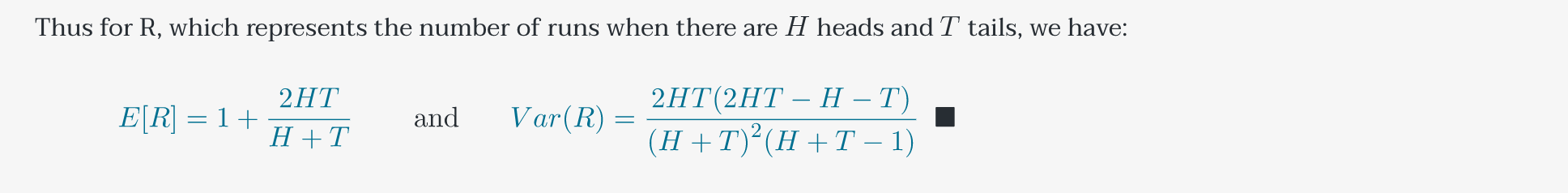
Thus for R, which represents the number of runs when there are heads and tails, we have:
![\begin{align*} {\color{MidnightBlue}{E[R] = 1 + \frac{2HT}{H+T} }} && \text{ and} && {{\color{MidnightBlue}{Var(R) = \frac{2HT(2HT-H-T)}{{(H+T)}^2(H+T-1)} }} \enspace \blacksquare} \end{align*}](https://www.rozmichelle.com/wp-content/ql-cache/quicklatex.com-e38aea8bde3643a165526713db3f4663_l3.png "Rendered by QuickLaTeX.com")
You can verify on the Wikipedia page that this is indeed the formula for the variance of the number of runs. This is probably the most rigorous math I’ve ever written for a proof! Whew! I hope this is useful, and if you stumbled across this page because you were looking for a proof of the variance of the number of runs, please give me credit! :)
At this point, one can use the normal distribution to see which sequence in the homework problem I provided is the true sequence of coin flips, but I’ll leave that as an exercise for the reader!
Powered by QuickLatex
You know what? This is pretty awesome. I mean the sheer breakdown and elaboration of each step is commendable. I googled, went through the nonparametric mammoths but no one offered anything. Zilch. Finally the main paper. Have a book that did kind of obscure proof beyond my brain. And the author seemed to have omitted them. In fact l, I reached here after going through google images. Helpful is a underrated word. Amazing. Best wishes.
P.S. The moment mathematician speak or write about ‘tedious proof’ it isn’t tedious at all. The question is: can a shorter proof be found?
Thanks, the book I just studied skipped the proof. I now know why. By the way, I am not a mathematician.
I have sent a reply earlier to Roslyn, I used her math for some algorithm in currency trading. Very useful and a persistent job she made with the proof.
Mama should be really proud.
This was super helpful, thank you!
My head hurts just trying to read this! Lol Very proud!
Mom